Calculation of Heat Demand#

Space and water heating for residential and commercial buildings amount to a third of the European Union’s total final energy consumption. Approximately 75% of the primary energy and 50% of the thermal energy are still produced by burning fossil fuels, leading to high greenhouse gas emissions in the heating sector. The transition from centralized fossil-fueled district heating systems such as coal or gas power plants to district heating systems sourced by renewable energies such as geothermal energy or more decentralized individual solutions for city districts makes it necessary to map the heat demand for a more accurate planning of power plant capabilities. In addition, heating and cooling plans become necessary according to directives of the European Union regarding energy efficiency to reach its aim of reducing greenhouse gas emissions by 55% of the 1990 levels by 2030.

Evaluating the heat demand (usually in MWh = Mega Watt Hours) on a national or regional scale, including space and water heating for each apartment or each building for every day of a year separately is from a perspective of resolution (spatial and temporal scale) and computing power not feasible. Therefore, heat demand maps summarize the heat demand on a lower spatial resolution (e.g. 100 m x 100 m raster) cumulated for one year (lower temporal resolution) for different sectors such as the residential and tertiary sectors. Maps for the industrial heat demand are not available as the input data is not publicly available or can be deduced from cultural data. Customized solutions are therefore necessary for this branch to reduce greenhouse gas emissions. Heat demand input values for the residential and commercial sectors are easily accessible and assessable. With the new directives regarding energy efficiency, it becomes necessary for every city or commune to evaluate their heat demand. And this is where PyHeatDemand comes into place. Combining the functionality of well-known geospatial Python libraries, the open-source package PyHeatDemand provides tools for public entities, researchers, or students for processing heat demand input data associated with an

administrative area (point or polygon), with a building footprint (polygon), with a street segment (line), or with an address directly provided in MWh but also as gas usage, district heating usage, or other sources of heat. The resulting heat demand map data can be analyzed using zonal statistics and can be compared to other administrative areas when working on regional or national scales. If heat demand maps already exist for a specific region, they can be analyzed using tools within PyHeatDemand. With PyHeatDemand, it has never been easier to create and analyze heat demand maps.

Demonstration Notebooks for Heat Demand Calculations#

Several Jupyter Notebooks are available that demonstrate the functionality of PyHeatDemand.

Examples

Processing Heat Demand Input Data#

Heat demand maps can be calculated using either a top-down approach or a bottom-up approach (Fig. 1). For the top-down approach, aggregated heat demand input data for a certain area will be distributed according to higher resolution data sets (e.g. population density, landuse, etc.). In contrast to that, the bottom-up approach allows aggregating heat demand of higher resolution data sets to a lower resolution (e.g. from building level to a 100 m x 100 m raster).

PyHeatDemand processes geospatial data such as vector data (points, lines, polygons), raster data or address data. Therefore, we make use of the functionality implemented in well-known geospatial packages such as GeoPandas, Rasterio, GeoPy, or OSMnx and their underlying dependencies such as Pandas, NumPy, Shapely, etc. In particular, we are utilizing the powerful implementation of Spatial Indices in GeoPandas allowing for processing speed-ups by orders of magnitudes compared to performing regular overlays and spatial joins for the processing of heat demand input data.

The creation of a heat demand map follows a general workflow (Fig. 2) followed by a data-category-specific workflow for five defined input data categories (Fig. 3 & 4). The different input data categories are listed in the table below.

Data category	Description
1	HD data provided as 100 m x 100 m raster or polygon grid with the same or in a different coordinate reference system
2	HD data provided as building footprints or street segments
3	HD data provided as a point or polygon layer, which contains the sum of the HD for regions of official administrative units
4	HD data provided in other data formats such as HD data associated with addresses
5	No HD data available for the region

Creating Global Mask#

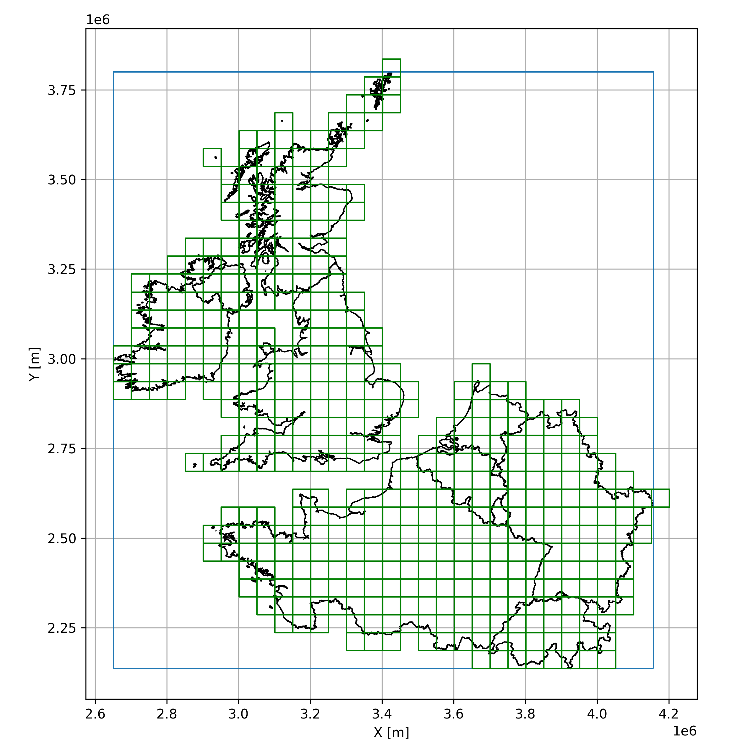
Depending on the scale of the heat demand map (local, regional, national, or even transnational), a global polygon mask is created from provided administrative boundaries with a cell size of 10 km by 10 km, for instance, and the target coordinate reference system. This mask is used to divide the study area into smaller chunks for a more reliable processing as only data within each mask will be processed separately. If necessary, the global mask will be cropped to the extent of the available heat demand input data.

# Creating global 10 km x 10 km mask and cropping it to the borders of the provided administrative areas.
# NB: The image below shows cells with a size of 50 km x 50 km for better visualization.
from pyheatdemand import processing
import geopandas as gpd

borders = gpd.read_file('path/to/borders.shp')
mask_10km = processing.create_polygon_mask(gdf=borders, step_size=10000, crop_gdf=True)

Creating Local Mask#

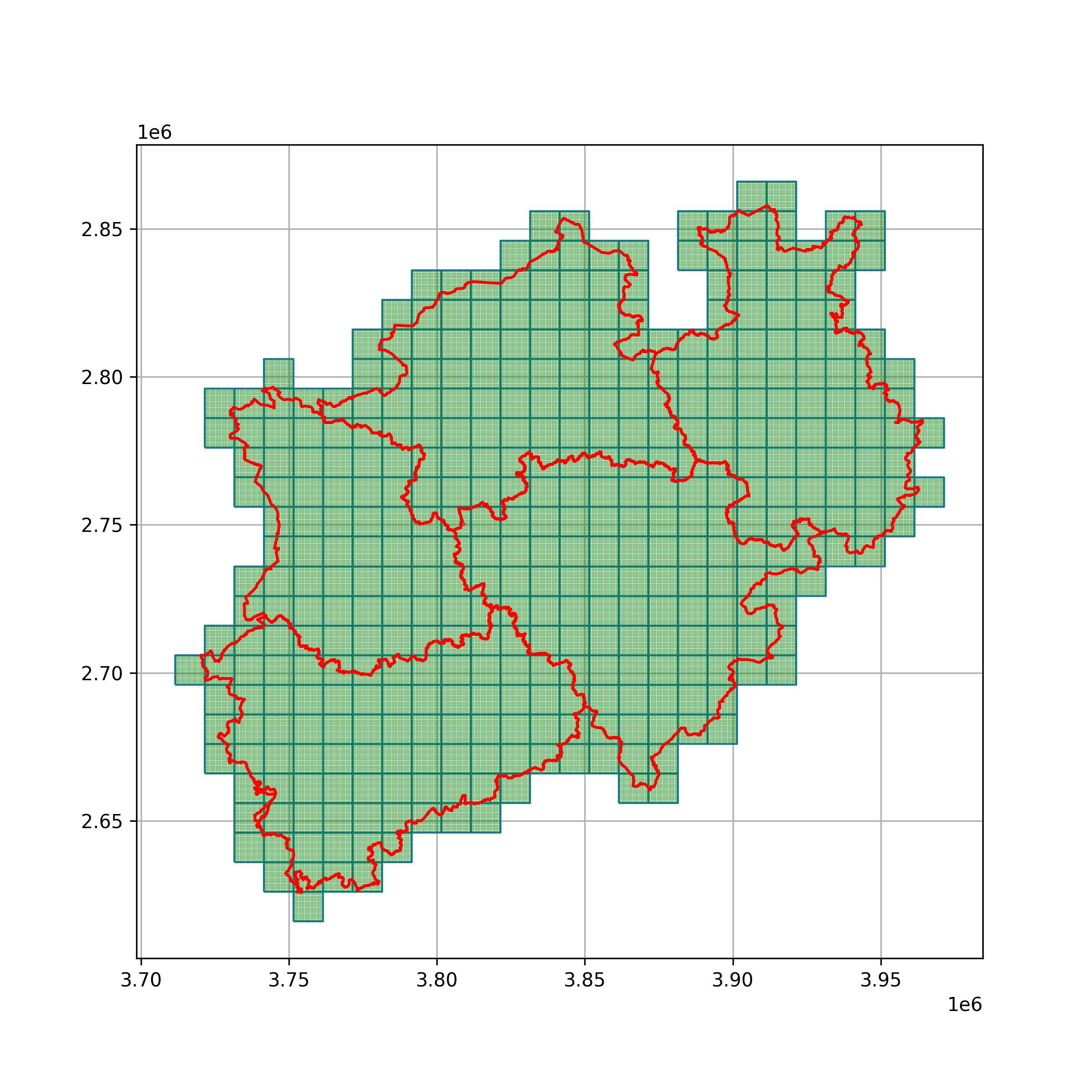
The global mask will be populated with polygons having already the final cell size such as 100 m x 100 m. Prior to that we are using a spatial join to crop the global mask to the extent of one administrative unit.

# Performing spatial join to crop global mask to outline of one administrative unit
outline_administrative_unit = gpd.read_file('path/to/outline.shp')
mask_10km_cropped = mask_10km.sjoin(outline_administrative_unit).reset_index(drop=True).drop('index_right', axis=1)
mask_10km_cropped = mask_10km_cropped.drop_duplicates().reset_index(drop=True)

# Creating local 100 m x 100 m mask for one of the administrative areas
mask_100m_cropped = [processing.create_polygon_mask(gdf=mask_10km[i:i+1],
                                               step_size=100,
                                               crop_gdf=True) for i in tqdm(range(len(mask_10km_cropped)))]
mask_100m = pd.concat(mask_100m_cropped)

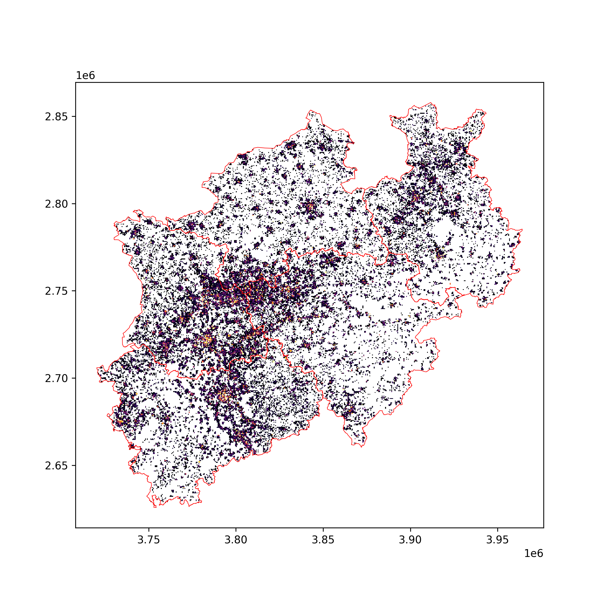
Calculating Heat Demand#

For each cell, the cumulated heat demand in each cell will be calculated.

gdf_hd = gpd.read_file('path/to/hd_data.shp')
heat_demand_list = [processing.calculate_hd(hd_gdf=gdf_hd, mask_gdf=mask_100m_cropped[i], hd_data_column='HD_column') for i in tqdm(range(len(mask_100m_cropped)))]
heat_demand = pd.concat(heat_demand_list).reset_index(drop=True)

Rasterizing Heat Demand#

The final polygon grid will be rasterized and merged with adjacent global cells to form a mosaic, the final heat demand map. If several input datasets are available for a region, i.e. different sources of energy, they can either be included in the calculation of the heat demand or the resulting rasters can be added to a final heat demand map.

processing.rasterize_gdf_hd(heat_demand,
                 path_out='path/to/heat_demand.tif',
                 crs = 'EPSG:3034',
                 xsize = 500,
                 ysize = 500)

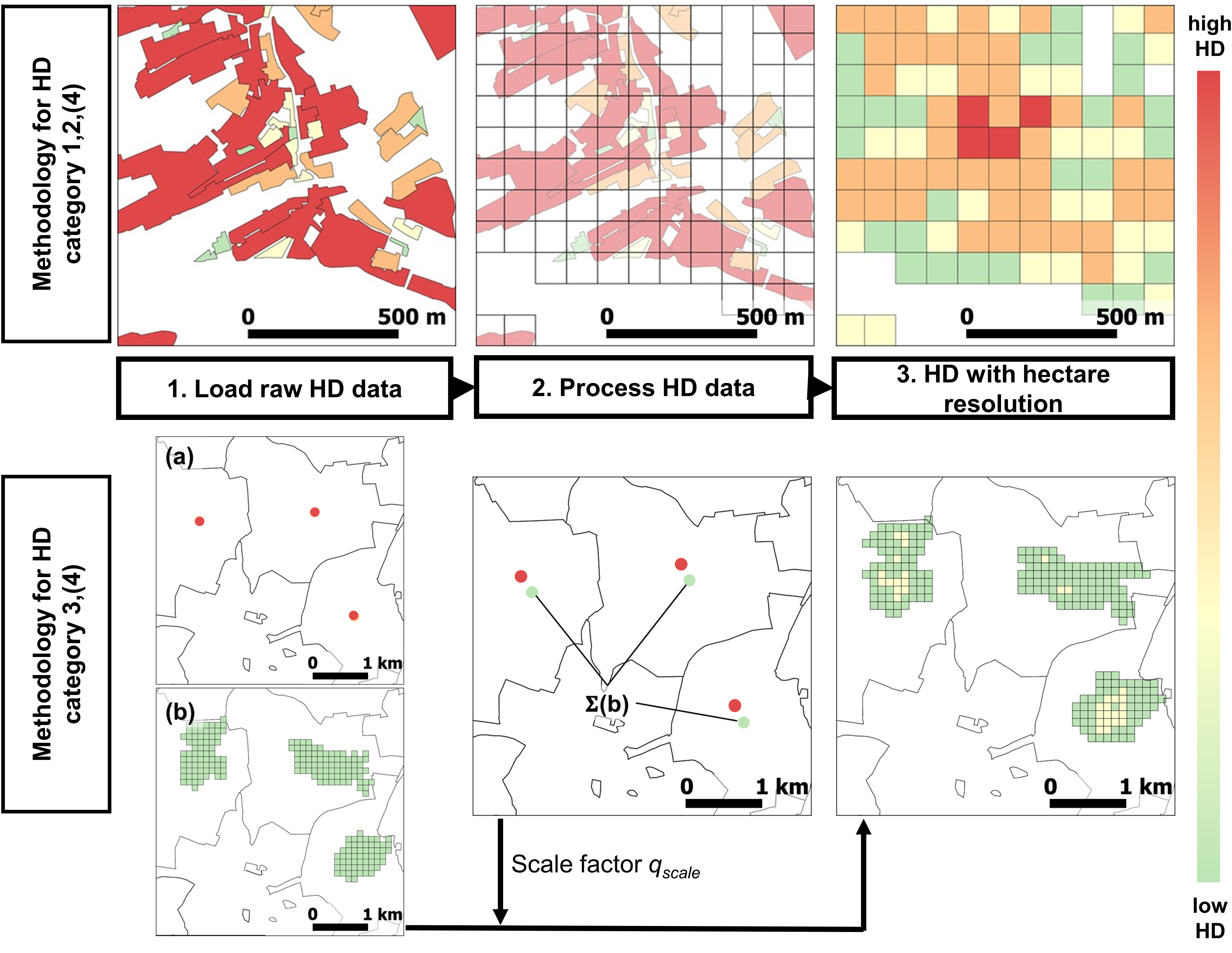
Processing data categories 1 and 2#

The data processing for data categories 1 and 2 are very similar (Fig. 3) and correspond to a bottom-up approach. In the case of a raster for category 1, the raster is converted into gridded polygons. Gridded polygons and building footprints are treated equally. The polygons containing the heat demand data are, if necessary, reprojected to the coordinate reference system and are overlain with the local mask (e.g. 100 m x 100 m cells). This cuts each heat demand polygon with the respective mask polygon. The heat demand of each subpolygon is proportional to its area compared to the area of the original polygon. The heat demand for all subpolygons in each cell is aggregated to result in the final heat demand for this cell.

Processing data category 3#

The data processing for data category 3 corresponds to a top-down approach. The heat demand represented as points for an administrative unit will be distributed across the area using higher-resolution data sets. In the case illustrated below, the distribution of Hotmaps data is used to distribute the available heat demands for the given administrative areas. For each administrative area, the provided total heat demand will distributed according to the share of each Hotmaps cell compared to the total Hotmaps heat demand of the respective area. The provided heat demand is now distributed across the cells and will treated from now on as category 1 or 2 input data to calculate the final heat demand map.

Processing data category 4#

The data processing for data category 4 corresponds to a bottom-up approach. Here, the addresses will be converted using the GeoPy geolocator to coordinates. Based on these, the building footprints are extracted from OpenStreet Maps using OSMnx. From there on, the data will be treated as data category 2.

Processing data category 5#

If no heat demand input data is available, the heat demand can be estimated using cultural data such as population density, landuse, and building-specific heat usage.

Processing Heat Demand Map Data#

Heat demand maps may contain millions of cells. Evaluating each cell would not be feasible. Therefore, PyHeatDemand utilizes the rasterstats package returning statistical values of the heat demand map for further analysis and results reporting.

gdf_stats = processing.calculate_zonal_stats('path/to/vector.shp',
                                             'path/to/heat_demand.tif',
                                             'EPSG:3034')
gdf_stats['coords'] = gdf_stats['geometry'].apply(lambda x: x.representative_point().coords[:])
gdf_stats['coords'] = [coords[0] for coords in gdf_stats['coords']]

PyHeatDemand - Processing Tool for Heat Demand Data

Calculation of Heat Demand

Contents