14 Refining Polygon Mask in high-density data areas
Contents
© Alexander Jüstel, Fraunhofer IEG, Institution for Energy Infrastructures and Geothermal Systems, RWTH Aachen University, GNU Lesser General Public License v3.0
14 Refining Polygon Mask in high-density data areas#
This notebook illustrates how to refine the polygon mask adding additional smaller polygons in high-density data areas.
Importing Libraries#
[1]:
import geopandas as gpd
import matplotlib.pyplot as plt

from pyheatdemand import processing
C:\Users\ale93371\Anaconda3\envs\pygeomechanical\lib\site-packages\numpy\_distributor_init.py:30: UserWarning: loaded more than 1 DLL from .libs:
C:\Users\ale93371\Anaconda3\envs\pygeomechanical\lib\site-packages\numpy\.libs\libopenblas.FB5AE2TYXYH2IJRDKGDGQ3XBKLKTF43H.gfortran-win_amd64.dll
C:\Users\ale93371\Anaconda3\envs\pygeomechanical\lib\site-packages\numpy\.libs\libopenblas64__v0.3.23-246-g3d31191b-gcc_10_3_0.dll
  warnings.warn("loaded more than 1 DLL from .libs:"
Loading Heat Demand Data#
The heat demand data utilized here can be downloaded from https://www.opengeodata.nrw.de/produkte/umwelt_klima/klima/raumwaermebedarfsmodell/.
[2]:
data = gpd.read_file('../../../test/data/HD_Aachen.shp')
data
[2]:
| OBJECTID | Fest_ID | spez_WB_HU | WB_HU | geometry | |
|---|---|---|---|---|---|
| 0 | 40.0 | 10000292 | 0.000000 | 0.000000 | POLYGON Z ((3729488.154 2675846.462 0.000, 372... |
| 1 | 41.0 | 10000293 | 0.000000 | 0.000000 | POLYGON Z ((3729487.353 2675845.779 0.000, 372... |
| 2 | 42.0 | 10000294 | 0.000000 | 0.000000 | POLYGON Z ((3729494.339 2675836.021 0.000, 372... |
| 3 | 43.0 | 10000295 | 0.000000 | 0.000000 | POLYGON Z ((3729493.781 2675833.641 0.000, 372... |
| 4 | 193.0 | 10001841 | 148.501500 | 237718.443608 | POLYGON Z ((3733429.797 2680405.183 0.000, 373... |
| ... | ... | ... | ... | ... | ... |
| 193361 | 2139002.0 | 249219 | 138.632092 | 16887.502341 | POLYGON Z ((3736358.156 2677252.398 0.000, 373... |
| 193362 | 2139003.0 | 249220 | 0.000000 | 0.000000 | POLYGON Z ((3736356.043 2677254.457 0.000, 373... |
| 193363 | 2139004.0 | 249221 | 0.000000 | 0.000000 | POLYGON Z ((3736364.286 2677250.432 0.000, 373... |
| 193364 | 3556749.0 | 1670883 | 0.000000 | 0.000000 | POLYGON Z ((3743898.286 2684862.227 0.000, 374... |
| 193365 | 3556750.0 | 1670884 | 0.000000 | 0.000000 | POLYGON Z ((3743906.306 2684864.617 0.000, 374... |
193366 rows × 5 columns
Creating the first mask#
The first mask is created as in any other tutorials before.
[3]:
grid = processing.create_polygon_mask(data, 1600)
grid
[3]:
| geometry | |
|---|---|
| 0 | POLYGON ((3726138.177 2668547.374, 3727738.177... |
| 1 | POLYGON ((3726138.177 2670147.374, 3727738.177... |
| 2 | POLYGON ((3726138.177 2671747.374, 3727738.177... |
| 3 | POLYGON ((3726138.177 2673347.374, 3727738.177... |
| 4 | POLYGON ((3726138.177 2674947.374, 3727738.177... |
| ... | ... |
| 127 | POLYGON ((3743738.177 2678147.374, 3745338.177... |
| 128 | POLYGON ((3743738.177 2679747.374, 3745338.177... |
| 129 | POLYGON ((3743738.177 2681347.374, 3745338.177... |
| 130 | POLYGON ((3743738.177 2682947.374, 3745338.177... |
| 131 | POLYGON ((3743738.177 2684547.374, 3745338.177... |
132 rows × 1 columns
Plotting the data and the mask#
[4]:
fig, ax = plt.subplots(1, figsize=(8,8))
grid.boundary.plot(ax=ax)
data.plot(ax=ax, column='WB_HU',legend=True, legend_kwds={'shrink':0.71, 'label': 'Heat Demand [kWh]'})
plt.xlabel('X [m]')
plt.ylabel('Y [m]')
[4]:
Text(36.347222222222214, 0.5, 'Y [m]')

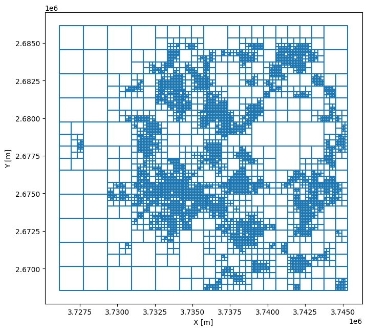
Refining the mask#
The mask is refined using the quad_tree_mask_refinement function that will be called four times here now.
[5]:
grid_ref1 = processing.refine_mask(grid, data, num_of_points=150, cell_size=800)
grid_ref2 = processing.refine_mask(grid_ref1, data, num_of_points=150, cell_size=400, area_limit=800*800)
grid_ref3 = processing.refine_mask(grid_ref2, data, num_of_points=100, cell_size=200, area_limit=400*400)
grid_ref4 = processing.refine_mask(grid_ref3, data, num_of_points=50, cell_size=100, area_limit=200*200)

fig, ax = plt.subplots(1, figsize=(8,8))
grid_ref4.boundary.plot(ax=ax)
plt.xlabel('X [m]')
plt.ylabel('Y [m]')
[5]:
Text(36.347222222222214, 0.5, 'Y [m]')
[6]:
grid_ref = processing.quad_tree_mask_refinement(grid, data, max_depth= 4, num_of_points = [150, 150, 100, 50])
grid_ref
[6]:
| geometry | |
|---|---|
| 0 | POLYGON ((3726138.177 2668547.374, 3727738.177... |
| 1 | POLYGON ((3726138.177 2670147.374, 3727738.177... |
| 2 | POLYGON ((3726138.177 2671747.374, 3727738.177... |
| 3 | POLYGON ((3726138.177 2673347.374, 3727738.177... |
| 4 | POLYGON ((3726138.177 2674947.374, 3727738.177... |
| ... | ... |
| 7030 | POLYGON ((3744238.177 2682047.374, 3744338.177... |
| 7031 | POLYGON ((3744338.177 2681747.374, 3744438.177... |
| 7032 | POLYGON ((3744338.177 2681847.374, 3744438.177... |
| 7033 | POLYGON ((3744438.177 2681747.374, 3744538.177... |
| 7034 | POLYGON ((3744438.177 2681847.374, 3744538.177... |
7035 rows × 1 columns
Calculating the Heat Demand#
[7]:
hd = processing.calculate_hd_sindex(hd_gdf=data,
                                    mask_gdf=grid_ref,
                                    hd_data_column='WB_HU')
hd
C:\Users\ale93371\Anaconda3\envs\pygeomechanical\lib\site-packages\geopandas\geodataframe.py:1538: SettingWithCopyWarning:
A value is trying to be set on a copy of a slice from a DataFrame.
Try using .loc[row_indexer,col_indexer] = value instead

See the caveats in the documentation: https://pandas.pydata.org/pandas-docs/stable/user_guide/indexing.html#returning-a-view-versus-a-copy
  super().__setitem__(key, value)
[7]:
| geometry | HD | |
|---|---|---|
| 0 | POLYGON ((3727738.177 2671747.374, 3729338.177... | 1.390320e+05 |
| 1 | POLYGON ((3727738.177 2673347.374, 3729338.177... | 9.952524e+05 |
| 2 | POLYGON ((3727738.177 2674947.374, 3729338.177... | 1.505710e+06 |
| 3 | POLYGON ((3727738.177 2676547.374, 3729338.177... | 7.207101e+05 |
| 4 | POLYGON ((3727738.177 2678147.374, 3729338.177... | 5.432950e+05 |
| ... | ... | ... |
| 6634 | POLYGON ((3744138.177 2681947.374, 3744238.177... | 3.471389e+05 |
| 6635 | POLYGON ((3744238.177 2681947.374, 3744338.177... | 1.249610e+05 |
| 6636 | POLYGON ((3744338.177 2681747.374, 3744438.177... | 7.055315e+05 |
| 6637 | POLYGON ((3744338.177 2681847.374, 3744438.177... | 0.000000e+00 |
| 6638 | POLYGON ((3744438.177 2681747.374, 3744538.177... | 2.969807e+05 |
6639 rows × 2 columns
Plotting the Heat Demand Map#
[8]:
fig, ax = plt.subplots(1, figsize=(8,8))
hd.plot(ax=ax, column='HD', cmap='inferno', vmax=1e6, legend=True, legend_kwds={'shrink':0.71, 'label': 'Heat Demand [MWh]'})
grid_ref.boundary.plot(ax=ax, color='black', linewidth=0.2)

plt.xlabel('X [m]')
plt.ylabel('Y [m]')
[8]:
Text(36.347222222222214, 0.5, 'Y [m]')

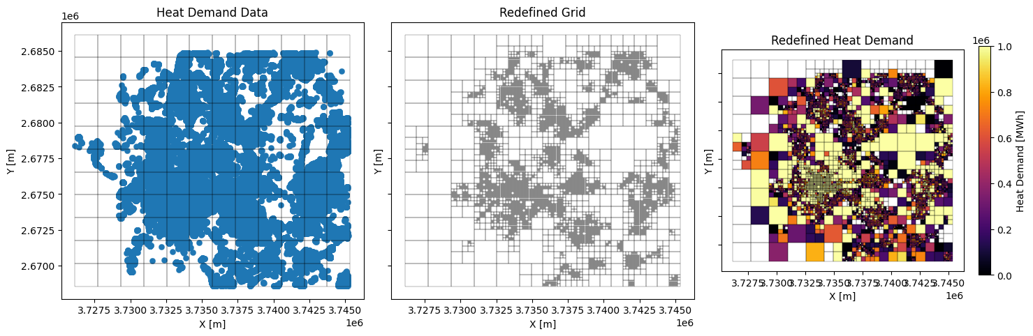
Plotting all maps together#
[9]:
fig, ax = plt.subplots(1, 3, figsize=(15,5), sharex=True, sharey=True)

grid.boundary.plot(ax=ax[0], color='black', linewidth=0.2)
data.plot(ax=ax[0], linewidth=0.2)
ax[0].set_xlabel('X [m]')
ax[0].set_ylabel('Y [m]')
ax[0].set_title('Heat Demand Data')

grid_ref.boundary.plot(ax=ax[1], color='black', linewidth=0.2)
ax[1].set_xlabel('X [m]')
ax[1].set_ylabel('Y [m]')
ax[1].set_title('Redefined Grid')

hd.plot(ax=ax[2], column='HD', cmap='inferno', vmax=1e6, legend=True, legend_kwds={'shrink':0.71, 'label': 'Heat Demand [MWh]'})
grid_ref.boundary.plot(ax=ax[2], color='black', linewidth=0.2)

ax[2].set_xlabel('X [m]')
ax[2].set_ylabel('Y [m]')
ax[2].set_title('Redefined Heat Demand')

plt.tight_layout()

# plt.savefig('../../../test/data/Grid_Refinement.png', dpi=600)
Histogram of the Heat Demand distribution#
[10]:
fig, ax = plt.subplots(3,2, figsize=(8,8))

ax[0][0].hist(hd['HD'][hd.area==10000].values, bins=25)
ax[0][1].hist(hd['HD'][hd.area==40000].values, bins=25)
ax[1][0].hist(hd['HD'][hd.area==160000].values, bins=25)
ax[1][1].hist(hd['HD'][hd.area==640000].values, bins=25)
ax[2][0].hist(hd['HD'][hd.area==2560000].values, bins=25)

ax[0][0].set_ylabel('Frequency')
ax[0][1].set_ylabel('Frequency')
ax[1][0].set_ylabel('Frequency')
ax[1][1].set_ylabel('Frequency')
ax[2][0].set_ylabel('Frequency')

ax[0][0].set_xlabel('Heat Demand [MWh]')
ax[0][1].set_xlabel('Heat Demand [MWh]')
ax[1][0].set_xlabel('Heat Demand [MWh]')
ax[1][1].set_xlabel('Heat Demand [MWh]')
ax[2][0].set_xlabel('Heat Demand [MWh]')

plt.tight_layout()
